OSPF Metric Cost

1. OSPF Metric Cost

OSPF uses the OSPF cost in order to calculate the best path to the destination.This cost comes from the speed your interfaces are operating at.
As you can see below, we have different types of interfaces, each with a cost number assigned.

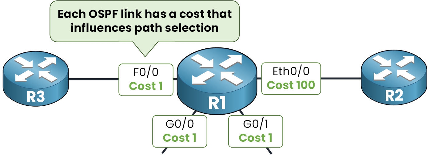
Figure 1 – OSPF cost per interface

To check the OSPF cost on our interfaces, we can use show ip ospf interface brief

R1# show ip ospf interface brief
Interface             PID   Area    IP Address/Mask            Cost  State  Nbrs
FastEthernet0/0         1   0     192.168.10.1/255.255.255.0   1     DR     0/0
GigabitEthernet0/0      1   0     192.168.12.1/255.255.255.0   1     DR     0/0
GigabitEthernet0/1      1   0     192.168.13.1/255.255.255.0   1     BDR    0/0
Ethernet0/0             1   0     192.168.11.1/255.255.255.0   100   DR     0/0

Here, we can clearly see that:

• FastEthernet and GigabitEthernet interfaces have a cost of 1

• Ethernet (10 Mbps) has a cost of 100

OSPF uses these values to evaluate the efficiency of each OSPF link.
The lower the cost, the more preferred the path.

2. How OSPF Selects the Path

In a typical OSPF network, to determine which path can be used to send packets to the destination, OSPF accumulates the cost of all the outgoing interfaces along the way and chooses the path with the lowest total cost.

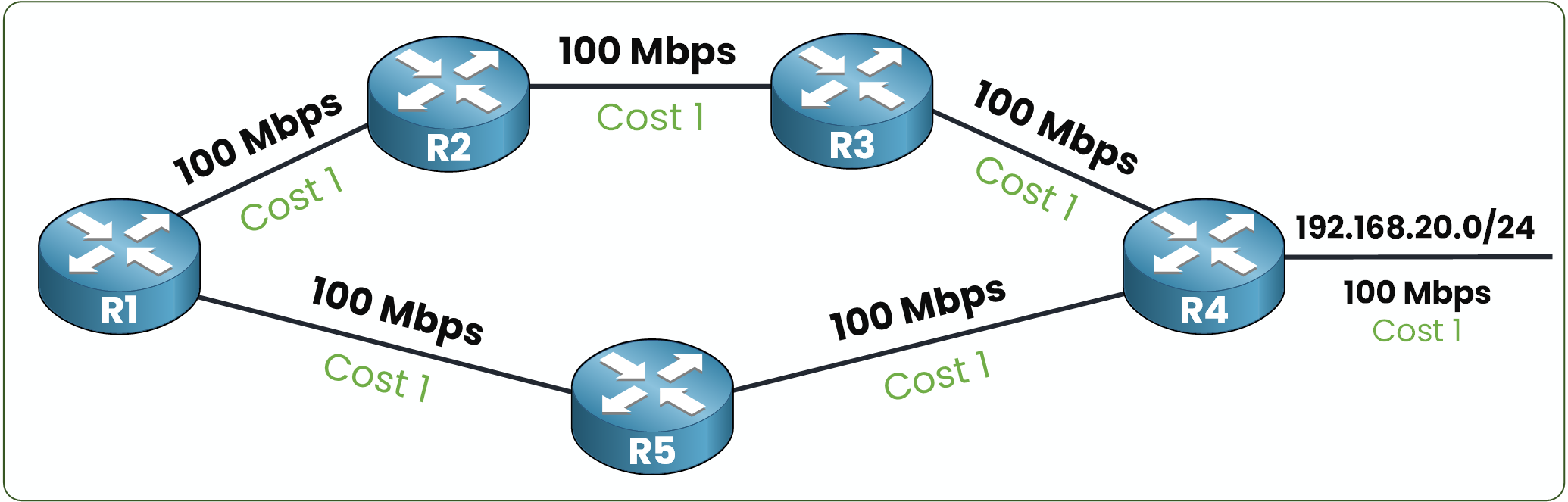
Figure 2 – OSPF Topology

In this example, we can check the route selected for 192.168.20.0/24 using:

R1# show ip route 192.168.20.0
Routing entry for 192.168.20.0/24
  Known via "ospf 1", distance 110, metric 3, type intra area
  Last update from 192.168.4.2 on GigabitEthernet0/1, 00:00:10 ago
  Routing Descriptor Blocks:
  * 192.168.4.2, from 192.168.20.1, 00:00:10 ago, via GigabitEthernet0/1
      Route metric is 3, traffic share count is 1

As you can see, the OSPF cost is 3 when using the path:
R1 -> R5 -> R4 -> 192.168.20.0/24
Cost: 1 + 1 + 1 = total cost 3

The alternative path is:
R1 -> R2 -> R3 -> R4 -> 192.168.20.0/24
Cost: 1 + 1 + 1 + 1 = total cost 4

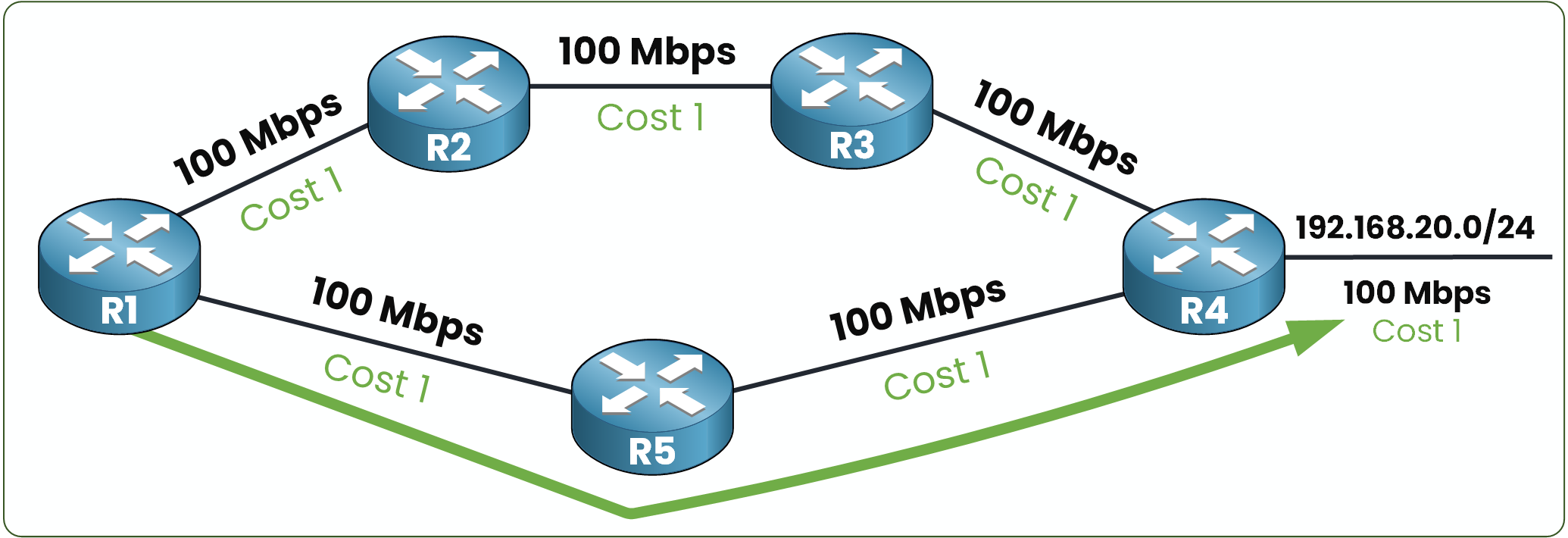
Figure 3 – OSPF chooses the path with the lowest total cost

OSPF selects the first path because it has the lowest metric.

3. How OSPF Calculates Cost

The OSPF cost is calculated using the following formula:

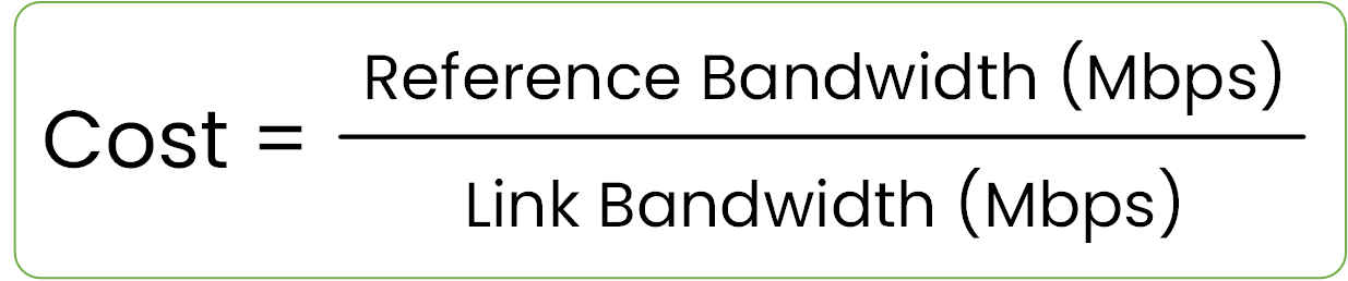
Figure 4 – Formula used to calculate OSPF cost

The reference bandwidth (in Mbps) is, by default, set to 100 Mbps.
The link bandwidth is determined by your interface type on your OSPF router.

Imagine you have a FastEthernet 100 Mbps interface:
→ The calculation is: Cost = 100 / 100 = 1

Pretty easy, right?

This default reference value was defined a long time ago, back when 100 Mbps was considered fast.
But today, network speeds have evolved a lot and that creates a problem.

Let’s look at the different interface types, their bandwidths, and their default OSPF costs:

OSPF Default Cost per Interface Type

Table 1 – Default OSPF cost values per interface type (based on 100 Mbps reference).

If you examine the table above, you'll notice a key detail: from 100 Mbps and more, the OSPF cost stays fixed at 1, even as interface speeds increase. That’s because the cost is calculated using the formula 100 / bandwidth, and OSPF cost only works with whole numbers.

When the result is a decimal, like 0.1 for a 1 Gbps link, it gets rounded up to 1. This means that whether you're using FastEthernet, Gigabit, or even 10 Gbps interfaces, OSPF sees them all as equal in cost.

The Problem With Default Cost

In this OSPF topology, all links with a bandwidth of 100 Mbps or more are assigned the same cost: 1.

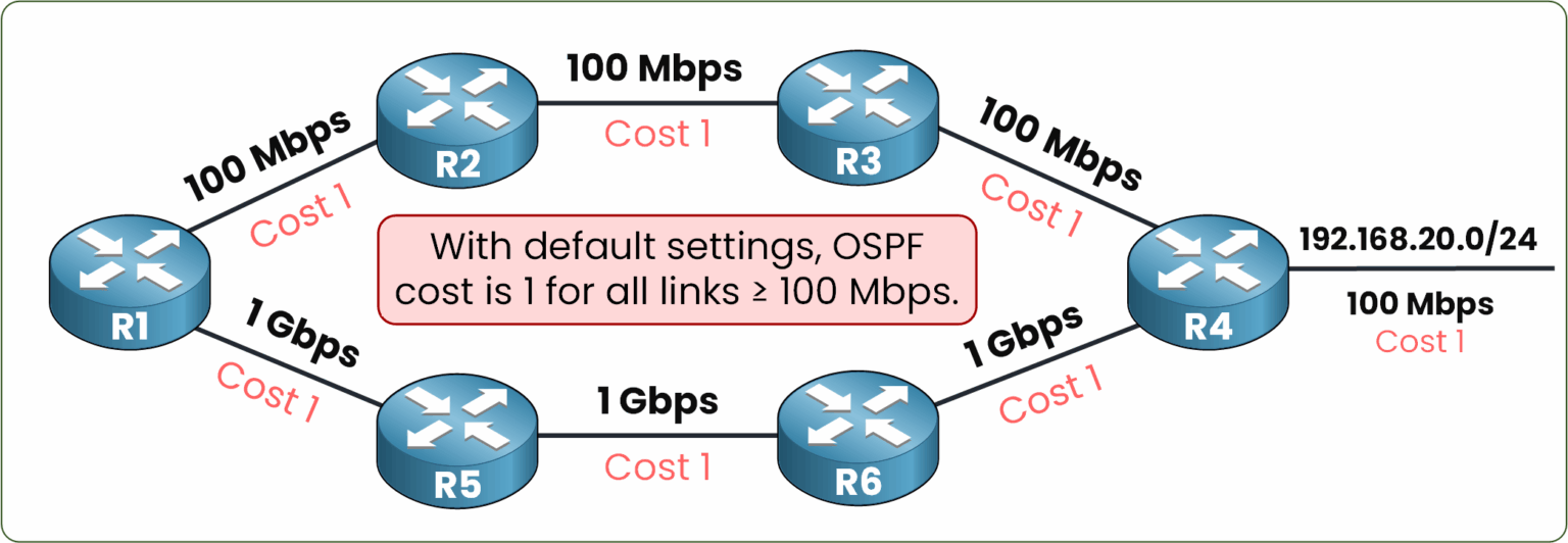
Figure 5 – OSPF sees 100 Mbps and 1 Gbps as equal

Here’s an example:
If we use 1 Gbps interfaces on the path R1 → R5 → R6 → R4, each link will have a cost of 1.

But a 100 Mbps link will also have a cost of 1, so OSPF can’t tell the difference between FastEthernet and Gigabit links.

In this case, OSPF will see two paths with the same total cost, and will load-balance the traffic between them.

R1# show ip route 192.168.20.0
Routing entry for 192.168.20.0/24
  Known via "ospf 1", distance 110, metric 4, type intra area
  Last update from 192.168.6.2 on GigabitEthernet0/1, 00:00:12 ago
  Routing Descriptor Blocks:
  * 192.168.6.2, from 192.168.20.1, 00:00:12 ago, via GigabitEthernet0/1
      Route metric is 4, traffic share count is 1
    192.168.2.2, from 192.168.20.1, 00:00:12 ago, via GigabitEthernet0/0
      Route metric is 4, traffic share count is 1

So R1 sends packets on both paths equally even if one uses Gigabit links and the other uses older 100 Mbps interfaces.

4. How to Tune OSPF Cost (3 Configurable Elements)

In order to make sure OSPF always uses the best path and is able to recognize and prioritize faster links, we can adjust three components of the OSPF cost calculation.

Figure 6 – Three elements can be tuned to influence OSPF cost

1. Reference Bandwidth

The first element we can modify is the reference bandwidth.
The best practice is to set the reference bandwidth to the highest bandwidth link in the OSPF network.

Since we have 1 Gigabit interfaces in our topology, we can set the reference bandwidth to 1000 Mbps using:

R1# conf t
Enter configuration commands, one per line. End with CNTL/Z.

R1(config)# router ospf 1
R1(config-router)# auto-cost reference-bandwidth ?
<1-4294967> The reference bandwidth in terms of Mbits per second

R1(config-router)# auto-cost reference-bandwidth 1000
% OSPF: Reference bandwidth is changed.
Please ensure reference bandwidth is consistent across all routers.

By using 1000 as the reference bandwidth:

Figure 7 – With 1000 Mbps as reference, OSPF can now differentiate link speeds

• A FastEthernet link of 100 Mbps will now have an OSPF cost of 10

• A GigabitEthernet link of 1000 Mbps will have a cost of 1

The reference bandwidth must be configured the same on all OSPF routers.

The 1 Gbps interface now has a cost of 1, which allows OSPF to correctly view it as a more efficient path.

If we retake our example, we can see that packets to 192.168.20.0/24 will now use: R1 → R5 → R6 → R4 → 192.168.20.0/24

Figure 8 – OSPF now selects the faster path thanks to the updated cost values

This path gives a cost of: 1 + 1 + 1 + 10 = 13

Whereas the previous path:

R1 → R2 → R3 → R4 → 192.168.20.0/24 has a total cost of 40.

R1#show ip route 192.168.20.0
Routing entry for 192.168.20.0/24
  Known via "ospf 1", distance 110, metric 13, type intra area
  Last update from 192.168.6.2 on GigabitEthernet0/1, 00:00:15 ago
  Routing Descriptor Blocks:
  * 192.168.6.2, from 192.168.20.1, 00:00:15 ago, via GigabitEthernet0/1
      Route metric is 103, traffic share count is 1

By modifying the reference bandwidth, you can adjust the OSPF cost in your topology. Always follow the best practice of setting the reference bandwidth to match the highest bandwidth interface in your network.

2. OSPF Cost (Per Interface)

The second parameter is the OSPF cost, and this one is modifiable per interface.
If you want to increase or decrease the cost of a specific link, you can set it manually.

Imagine we are on R1, and we want to increase the cost of G0/1 (which is the link to R5) to 100.
We can use the command ip ospf cost :

R1(config)# interface GigabitEthernet0/1
R1(config-if)# ip ospf cost ?
  <1-65535>  Cost

R1(config-if)# ip ospf cost 100

By doing this, OSPF will now prefer the path: R1 → R2 → R3 → R4 → 192.168.20.0/24

Figure 9 – R1 now prefers the upper path due to the manual cost set to 100

Because its total cost is 40, while the other path through R5 now has a cost of 112.

To verify the change, we can use the command: show ip ospf interface brief

R1#show ip ospf interface brief 

Interface           PID   Area    IP Address/Mask           Cost  State  Nbrs F/C
GigabitEthernet0/0    1     0     192.168.1.1/255.255.255.0   10     DR     0/0
GigabitEthernet0/1    1     0     192.168.4.1/255.255.255.0   100     DR     0/0

Here we are the cost is now 100 for interface G0/1.

3. Interface Bandwidth

The last element we can modify is the interface bandwidth.

Figure 10 – Link bandwidth can be modified manually.

On Cisco IOS, you can manually configure the bandwidth value of a link using the bandwidth command (in kilobits) under interface configuration mode.

For example, imagine we are using a GigabitEthernet interface (1 Gbps = 1,000 Mbps).
We can simulate that the interface operates at 100 Mbps, which is equivalent to 100,000 kilobits.

R1(config)# int g0/1
R1(config-if)# bandwidth ?
<1-10000000> Bandwidth in kilobits

R1(config-if)# bandwidth 1000000

Let’s verify it:

R1# show interfaces g0/1
GigabitEthernet0/1 is up, line protocol is up (connected)
Hardware is CN Gigabit Ethernet, address is 0002.1643.9701 (bia 0002.1643.9701)
Internet address is 192.168.4.1/24
MTU 1500 bytes, BW 100000 Kbit, DLY 10 usec,
reliability 255/255, txload 1/255, rxload 1/255
Encapsulation ARPA, loopback not set
Keepalive set (10 sec)
Full-duplex, 100Mb/s, media type is RJ45
output flow-control is unsupported, input flow-control is unsupported
ARP type: ARPA, ARP Timeout 04:00:00,
Last input 00:00:08, output 00:00:05, output hang never
Last clearing of "show interface" counters never
Input queue: 0/75/0 (size/max/drops); Total output drops: 0
Queueing strategy: fifo
Output queue :0/40 (size/max)
5 minute input rate 54 bits/sec, 0 packets/sec
5 minute output rate 54 bits/sec, 0 packets/sec
156 packets input, 11332 bytes, 0 no buffer
Received 0 broadcasts, 0 runts, 0 giants, 0 throttles
0 input errors, 0 CRC, 0 frame, 0 overrun, 0 ignored, 0 abort
0 watchdog, 1017 multicast, 0 pause input
0 input packets with dribble condition detected
151 packets output, 10708 bytes, 0 underruns
0 output errors, 0 collisions, 1 interface resets
0 unknown protocol drops
0 babbles, 0 late collision, 0 deferred
0 lost carrier, 0 no carrier
0 output buffer failures, 0 output buffers swapped out

By doing this, OSPF will now calculate the cost using:

Cost = Reference Bandwidth (Mbps) / Interface Bandwidth (Mbps)Cost = 1000 / 100 = 10

Now, if we check the OSPF cost:

R1# show ip ospf interface brief

Interface              PID   Area    IP Address/Mask            Cost  State  Nbrs
GigabitEthernet0/0       1   0     192.168.12.1/255.255.255.0    1     DR     0/0
GigabitEthernet0/1       1   0     192.168.4.1/255.255.255.0     10    BDR    0/0

Keep in mind:
This command does not change the real bandwidth of the interface, it only tells the OSPF process how to calculate the cost.

Summary

• OSPF chooses paths based on cumulative interface cost.

• The default cost logic is outdated because it assumes 100 Mbps is the top speed.

• You can fix this by:

  • Setting the reference bandwidth correctly

  • Manually adjusting interface cost

  • Changing the interface bandwidth value (affects OSPF cost calculation only)