EIGRP Wide Metrics

In the previous lesson, you saw how EIGRP calculates the classic metric from the minimum bandwidth and the total delay.
That formula works well until the links become very fast.

Classic EIGRP was originally designed when high-speed interfaces were limited to 1 Gbps.

At that time, the metric formula scaled correctly for available link speeds.
However, modern networks now operate with 10 Gbps, 20 Gbps, 40 Gbps, and even 100 Gbps interfaces.

This is where the limitation appears.

A 10 Gbps Link vs a 20 Gbps Link

In this topology, one path uses a 10 Gbps link and another uses a 20 Gbps link.

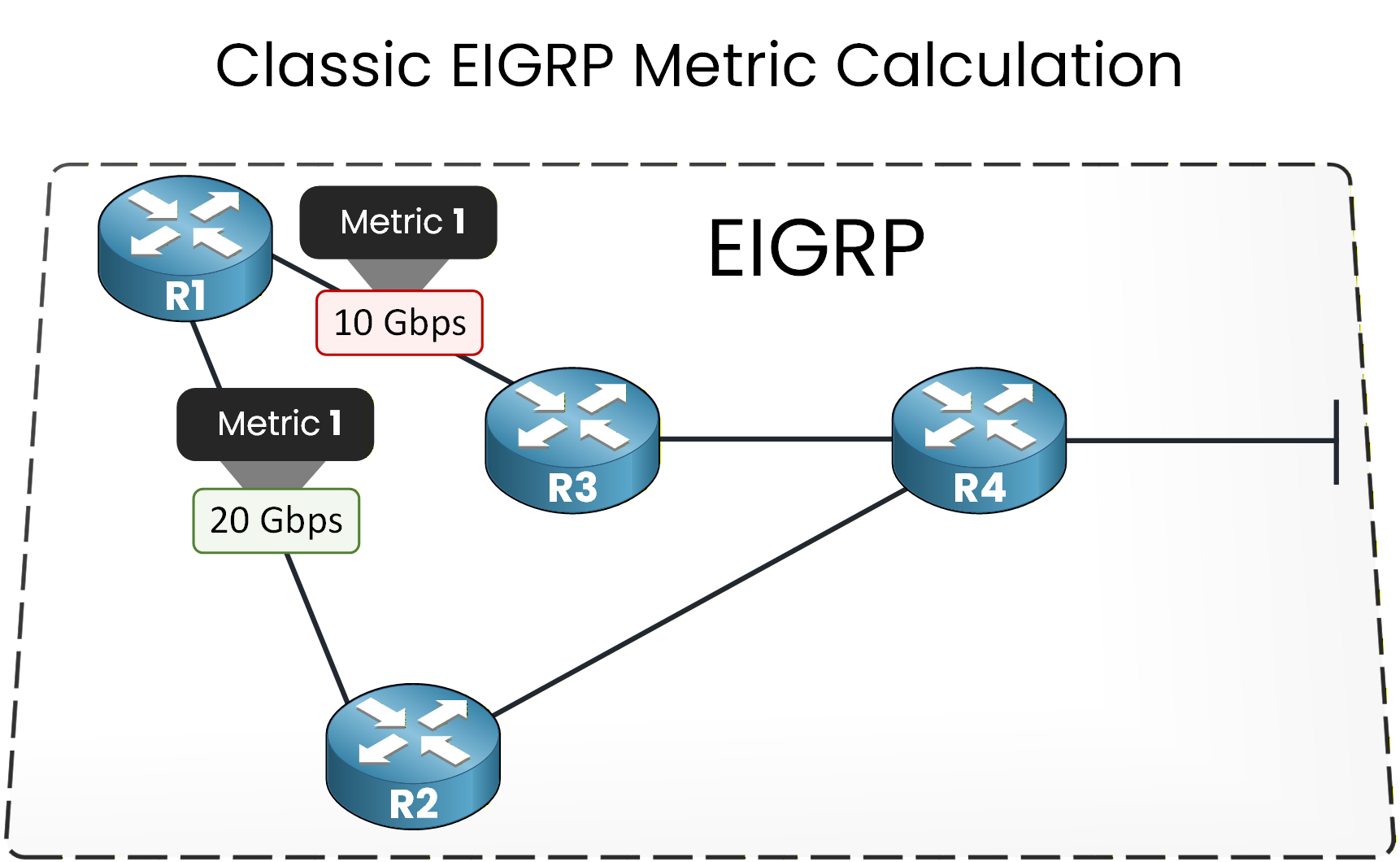
Figure 1 – Classic EIGRP metric where 10G and 20G links produce the same cost

Even though 20 Gbps is twice as fast, the calculated metric is identical.
From EIGRP's perspective, both paths have the same cost.

The Bandwidth Term

The reason lies in how the bandwidth term is calculated in the classic formula:

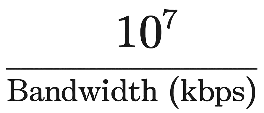
Figure 2 – Classic EIGRP Bandwidth Term Calculation

The key limitation is that this value cannot go below 1.
Once the result reaches 1, it is treated as the minimum possible value.

The Bandwidth Term per Link Speed

Table 1 - Classic EIGRP Metric Saturation at 10 Gbps

If you examine the table above, you can clearly see that starting at 10 Gbps, classic EIGRP can no longer differentiate higher speeds.

• 1 Gbps → bandwidth term = 10 → final metric = 2816

• 5 Gbps → bandwidth term = 2 → final metric = 768

• 10 Gbps → bandwidth term = 1 → final metric = 512

• 20 Gbps → calculated value = 0.5 → forced to 1 → final metric = 512

• 40 Gbps → calculated value = 0.25 → forced to 1 → final metric = 512

• 100 Gbps → calculated value = 0.1 → forced to 1 → final metric = 512

From 10 Gbps and above, the bandwidth component is effectively fixed at 1.

As a result:
(1 + 1) × 256 = 512

No matter how fast the link becomes beyond 10 Gbps, the metric remains the same.
Therefore, classic EIGRP cannot differentiate links faster than 10 Gbps when delay is identical.

Transition to Wide Metrics

This limitation led to the introduction of EIGRP Wide Metrics, which extend the scaling mechanism and allow proper differentiation of modern high-speed interfaces.

The next section explains how Wide Metrics solve this limitation.

With Wide Metrics, the bandwidth component continues scaling as link speed increases.

Wide Metric Formula

You are not required to memorize the formula.

Figure 3 – Detailed wide metric formula

The wide metric introduces:

• A larger multiplier (65,535 instead of 256)

• More precise bandwidth calculation

• Latency expressed with greater accuracy

The key takeaway:

The bandwidth value no longer bottoms out at 1.

Practical Comparison

With Wide Metrics enabled, high-speed interfaces produce distinct metric values.

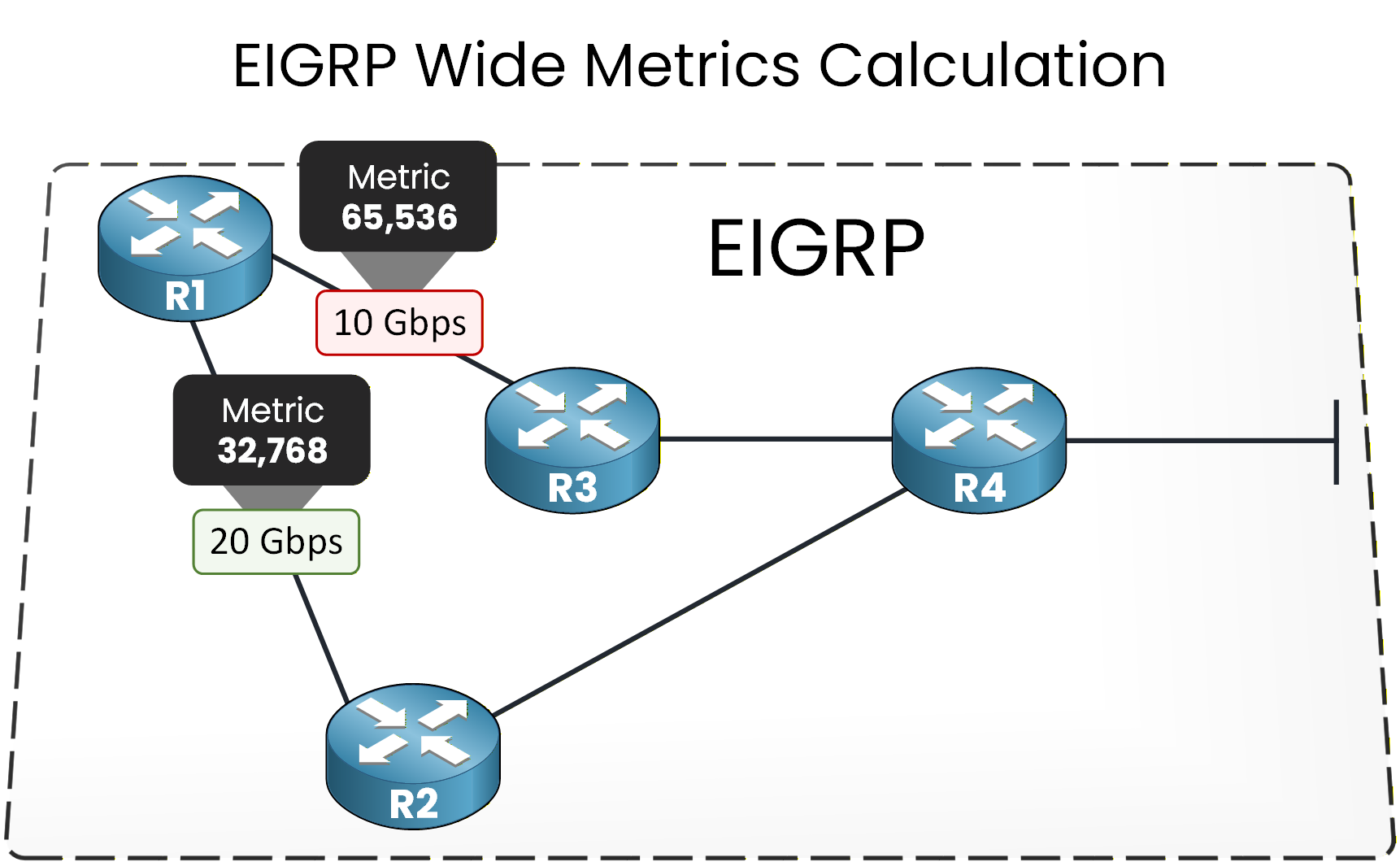
Figure 4 – Wide metrics calculation differentiating high-speed links

Classic vs Wide Metric Scaling Comparison

Table 2 – Classic vs Wide EIGRP Metric Scaling on High-Speed Links

We observe:

• In classic EIGRP, 10 Gbps and above produce identical bandwidth terms.

• In Wide Metrics, the bandwidth term continues decreasing as speed increases.

Wide Metrics restore proper path differentiation in modern high-speed networks.

In the next lesson, a router compares two of these metrics toward the same network and picks its best path.